Welcome!
⚠️ In Progress! ⚠️
Machine Learning Fundamentals
K-Nearest Neighbours (KNN)
What's the Problem?
Congrats! You just manufactured your very own car, the WMB X5 😱👑. You think it's a pretty fancy car, so you'd like to try to sell it by sending ads to people who might be interested in buying a new vehicle. Fortunately, your friend Zark Muckerberg runs a social network and collects a lot of data on his users. He runs a small survey to see who'd be interested in buying a new car and sends you the results.
| User ID | Gender | Age | Salary | Interested |
|---|---|---|---|---|
| 6939211 | Male | 25 | 83250 | No |
| 9177299 | Male | 37 | 76234 | No |
| 9323247 | Female | 70 | 93668 | Yes |
| ... | ||||
| 451242142 | Female | 32 | 70904 | No |
For each user on the social network, you can now decide whether to send an ad to them. What you effectively want then is a model that can use the data your friend gave you to take some unseen user data like
| User ID | Gender | Age | Salary |
|---|---|---|---|
| 631222142 | Female | 43 | 90090 |
And predict whether that user would be interested in a new car.
What is K-Nearest Neighbours (KNN)?
KNN is a very simple supervised machine learning algorithm whose logic can effectively be summarised as "Birds of a feather flock together". The idea is to plot all of your data as points in some multivariable space. Then, for each new point of unknown data, we find the K closest data points, and whatever is the most common label among those is the predicted label of our unknown point.
But, how do we measure distance? For now, we'll just use Euclidean distance, which is the distance between two points (or vectors) formula that you learnt in high school.
\[ \text{distance}(x, y) = \sqrt{\sum_{i=1}^{n}(y_i - x_i)^2} \]
Which might look more familiar in 2D
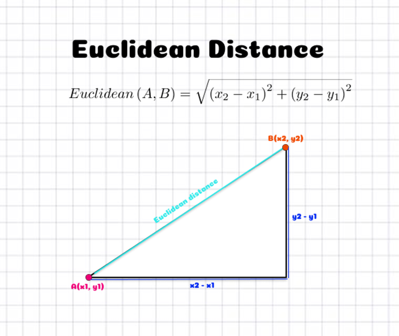
So, in the case of our car advertisement, we might decide to use the Age and Salary of users as our training data, and our label will simply be whether they are interested or not interested in a new car. Using the KNN algorithm with the query data above, we thus predict the user is not interested in a new car!
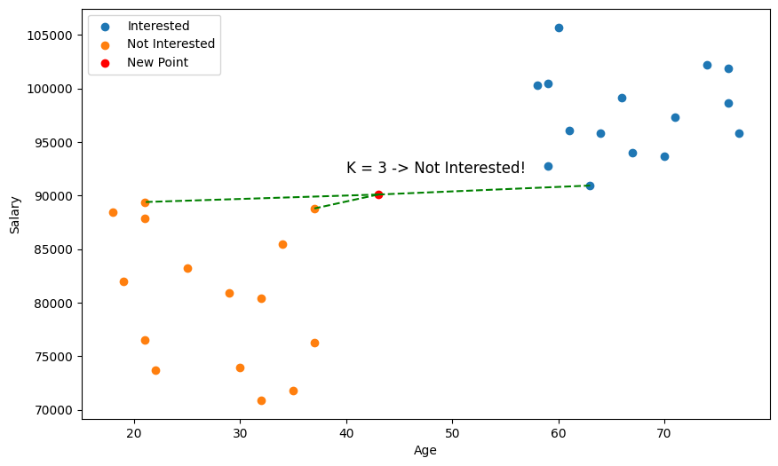
But wait a minute 🤔, just by eyeballing the scatter plot, it seems we didn't pick the closest points?
This is why something called feature scaling is important. With distance based algorithms like KNN, features (variables) with bigger numbers can disproportionately influence the distance calculation. Here, salary is going to be of much larger magnitude than age, so our distance metric is going to be more biased towards salary. So, we need to scale our values so that they're comparable.
Two common feature scaling methods are Min-Max scaling and Standardisation.
Min-Max scaling squeezes values into a specific range, usually [0, 1], and is calculated using the formula:
\[ x_{scaled} = \frac{x - x_{min}}{x_{max} - x_{min}} \]
Standardisation does a similar thing by centering the values around the mean (transformed to 0) and scaling them based on the standard deviation. While this doesn't limit the values to a range, this will usually place them around -1 to 1.
\[ x_{scaled} = \frac{x - \text{mean}}{\text{standard deviation}} = \frac{x - \mu}{\sigma} \]
Usually, you should try both to see which one works better, but we're going to go ahead and use Standardisation.
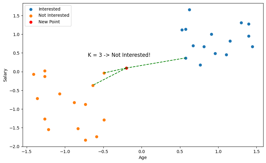
Exercise
Your task is to implement a KNN classifier. You must implement euclidean_distance(), fit() which prepares the training data for use in the model, _predict() which returns the KNN classification for a single data point, and predict() which returns the classification for an array of data points.
Inputs - euclidean_distance():
x1andx2are both single data points represented as NumPy arrays. For example,x1 = [1, 1, 0]andx2 = [3, 3, 4].
Inputs - fit():
Xis a NumPy NDArray (matrix) of data points such as[[1, 1, 0], [0, 0.5, 3], [0.7, 0.9, 0.3]], representing the training data (e.g., a set of coordinates [age, salary] for numerous users).yis a NumPy NDArray (vector) of labels such as["Yes", "No", "Yes"], representing the labels/classification of the training data (e.g., whether each corresponding user is interested or not interested in a car).
Inputs - _predict():
xis a NumPy NDArray (vector) such as[1, 1, 0]representing a single data point for which we should return the predicted label.
Inputs - predict():
Xis a NumPy NDArray (matrix) of data points such as[[1, 1, 0], [0, 0.5, 3], [0.7, 0.9, 0.3]], representing a set of points we want to predict labels for.
Note: type hints are used throughout the training exercises, but this is generally not common for most development in data science. Typically, type hints will be omitted during initial data exploration to save time, and only implemented during collaboration or for production level code.
Extra Reading: Distance Metrics
The most intuitive and natural way to represent distance between your data points is Euclidean distance, but we could actually use a whole range of different functions to calculate the distance between two data points. Why might we want this though?
One reason is that we want to represent the distance between two data points that are not necessarily numerical. We could be dealing with categorical data, in which case Hamming distance is usually most appropriate, or we might want to compare strings in which case Levenshtein distance could help us.
Another reason is that each distance metric makes assumptions about our data. For instance, the Euclidean distance treats all dimensions equally, so it's sensitive to extreme differences in a single attribute. So, if you were dealing with data points with 1000 different variables, and 999 of them were close to label A, but 1 was a really large number, completely outside of the standardisation, then you might end up classifying it as label B, or C, or D, etc. In cases like this Minkowski distance might be desirable.
Extra Reading: K Values
What value should we pick for k? In our examples, we used 3, but we could have just as easily chosen 5, 6, or 100. In general, the choice of k is quite critical and it should be tested for each dataset. Small values of k mean that noise in your dataset will have a higher influence on the result. Large values of k slow down each prediction and decrease the effect of relying on the labels of nearest neighbours. There are even very good arguments that k should be the square root of the size of the data.
Linear Regression
What's the Problem?
Think you're good at marketing 🤔? No? Well, too bad. You're now the director of a major marketing firm and you're trying to develop an equation that will let you predict how many sales a company will make based on how much it spends on advertising. You currently have access to a dataset like this
| Company | Social Media ($) | TV ($) | Billboards ($) | Sales ($) |
|---|---|---|---|---|
| Micro$oft | 23.32 | 8.43 | 24.25 | 1367.71 |
| Adobe | 15.82 | 4.15 | 26.94 | 508.51 |
| Fenty | 24.99 | 10.04 | 20.51 | 785.73 |
| Chanel | 25.99 | 23.32 | 13.52 | 1090.09 |
| Riot Games | 26.19 | 19.12 | 8.52 | 651.36 |
Since the data is continuous and you think the output has a constant slope, what you effectively want is a line of best fit. So, using our data, can we generate a function like this?
\[ \text{Sales} = w_1 \text{Social Media} + w_2\text{TV} + w_3\text{Billboards} \]
What is a Linear Regression?
A Linear Regression refers to a set of supervised learning algorithms which work out the coefficients for a linear combination of parameters, such that we minimise some cost function. This might sound like a broad statement, but that's because linear regression is a huge topic with a lot of depth and alternative algorithms. But, for now, what we want is to optimise an equation like
\[ \hat{y} = b +\sum_{i=1}^{n}w_ix_i \]
Where \(\hat{y}\) represents our ouput, and \( w_i \) represents the coefficient for the variable (feature) \(x_i\) we wish to factor into our equation. Often, these coefficients are called the weights of your model. As you can see, this means we have \(n\) variables in our equation, and \( n \) weights. But hold on, what's \(b\) 🤔? This is our bias term (sometimes just referred to as \(w_0\)), which just offsets all the predictions we make. If you think in terms of a line of best fit, this is just where our line intercepts the output axis.
We'll stick to this notation, but just so you're aware, there are many differing notations for the equation above.
\[ \hat{y} = \beta_0 + \sum_{i=1}^{p}\beta_i x_i \]
\[ h_\theta(\overrightarrow{x^{(i)}}) = \theta_0 + \sum_{z=1}^{n}\theta_z x_z^{(i)} \]
Loss Function
But what are we optimising our weights for? What we need is a cost function, which measures how bad our weights are at predicting the output of the training set. This is often also called a loss function or a criterion.
In our example, we'll use the Mean Squared Error (MSE) as our cost function. MSE measures the average of the square differences between the predicted value and the actual value. The output is just a single number representing the cost associated with our current weights. So, lower = better 🤓!
\[ \text{MSE} = \frac{1}{N} \sum_{i=1}^{n}(y_i - \hat{y_i})^2 \]
\[ \text{MSE} = \frac{1}{N} \sum_{i=1}^{n}(\underset{\text{actual output for the ith data point}}{\underbrace{y_i}} - \underset{\text{predicted output for the ith data point}}{\underbrace{\hat{y_i}}})^2 \]
Before we go any further, let's just recontextualise this in terms of our advertising example. We'll first only consider 1 variable, let's say TV Advertising, and we'll call it \(x \) just to keep things simple. Here \(x_i \) refers to the TV Advertising expenditure for the \(ith \) row on our table.
\[ \text{Sales}_i = wx_i + b \]
We'll thus rewrite our loss function accordingly
\[ \mathcal{L}(w, b) = \frac{1}{N}\sum_{i=1}^{n}(y_i - \text{Sales}_i)^2 \]
\[ \mathcal{L}(w, b) = \frac{1}{N}\sum_{i=1}^{n}(y_i - (wx_i + b))^2 \]
Gradient Descent
Okay, so we have a function (Sales) with parameters \(w\) and \(b\), and a loss/cost function, \(\mathcal{L}\) that measures how poorly our current choices of \(w\) and \(b\) predict the training data. To improve \(w\) and \(b\), or equivalently to minimise \(\mathcal{L}\), we'll use a technique called Gradient Descent.
Gradient Descent is an iterative optimisation algorithm used to minimise the loss function. Here's how it works:
- Evaluate the Error: Calculate the current error using the loss function \(\mathcal{L}\) with the current values of \(w\) and \(b\).
- Compute the Gradient: Find the derivative of the loss function \(\mathcal{L}\) with respect to \(w\) and \(b\). This gives us the gradient, which indicates the direction of the steepest increase in the error.
- Update Parameters: Adjust \(w\) and \(b\) by moving them in the direction opposite to the gradient. We move in the opposite direction because the gradient points to where the error increases, so moving the opposite way will help reduce the error.
By repeatedly applying these steps, we gradually adjust \(w\) and \(b\) to minimise the loss function \(\mathcal{L}\), thereby improving our linear regression.
A very common way to think about gradient descent is like a ball rolling down a mountain. Our loss function is some mountainous terrain, and the coordinates of its current position corresponds to the parameters of our model. We'd like to find the point on the mountain with the lowest elevation. So, what we'll do is look at the direction where the increase in elevation is steepest and push our ball in the opposite direction. If we keep doing this in small bursts, hopefully we'll find the point of lowest elevation, or at least low enough.
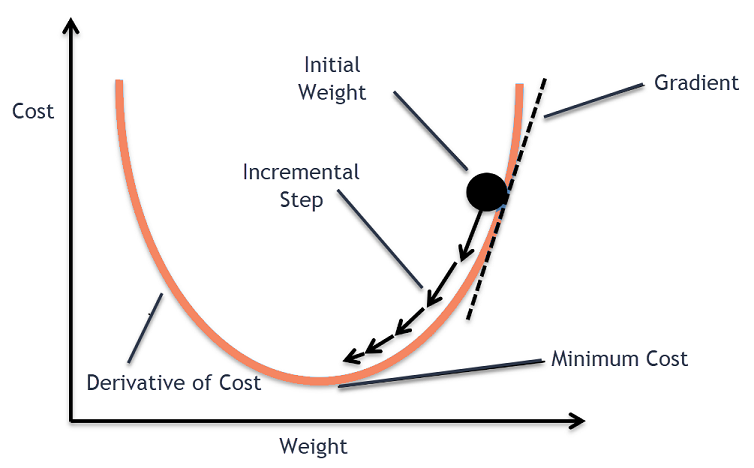
So how do we find the derivative of \(\mathcal{L}\) with respect to \(w\) and \(b\)? Since we need to consider \(w\) and \(b\) independently, we need to find their partial derivatives. We can find their partial derivatives by noticing that \((y_i - (wx_i + b))^2\) is really 2 nested functions: the inner function \(y_i - (wx_i + b)\) and the outer function \(u^2\). This means, we can just use the Chain rule that you learnt in high school!
Returning to our loss function:
\[ \mathcal{L}(w, b) = \frac{1}{N}\sum_{i=1}^{n}(y_i - (wx_i + b))^2 \]
Step 1: Because the derivative of a sum is the sum of the derivatives, we can focus on finding the derivative of each \((y_i - (wx_i + b))^2\). So define \(\mathcal{L}_i\):
\[ \mathcal{L}_i(w, b) = (y_i - (wx_i + b))^2 \]
Step 2: Differentiate with respect to \(w\):
Using the chain rule, let \(u = y_i - (wx_i + b)\). Then \(\mathcal{L}_i (w, b) = u^2\).
\[ \frac{\partial \mathcal{L_i}}{\partial w} = \frac{\partial \mathcal{L_i}}{\partial u} \frac{\partial u}{\partial w} \]
First, compute \(\frac{\partial \mathcal{L_i}}{\partial u}\):
\[ \frac{\partial \mathcal{L_i}}{\partial u} = 2u = 2(y_i - (wx_i + b)) \]
Then, compute \(\frac{\partial u}{\partial w}\):
\[ \frac{\partial u}{\partial w} = -x_i \]
Combine these results and simplify:
\[ \frac{\partial \mathcal{L_i}}{\partial w} = 2(y_i - (wx_i + b)) \times -x_i \]
\[ \frac{\partial \mathcal{L_i}}{\partial w} = -2x_i(y_i - (wx_i + b)) \]
Step 3: Differentiate with respect to \(b\):
Using the chain rule again, let \(u = y_i - (wx_i + b)\). Then \(\mathcal{L}_i (w, b) = u^2\).
\[ \frac{\partial \mathcal{L_i}}{\partial b} = \frac{\partial \mathcal{L_i}}{\partial u} \frac{\partial u}{\partial b} \]
First, compute \(\frac{\partial \mathcal{L_i}}{\partial u}\) (same as before):
\[ \frac{\partial \mathcal{L_i}}{\partial u} = 2u = 2(y_i - (wx_i + b)) \]
Then, compute \(\frac{\partial u}{\partial b}\):
\[ \frac{\partial u}{\partial b} = -1 \]
Combine these results and simplify:
\[ \frac{\partial \mathcal{L_i}}{\partial b} = -2(y_i - (wx_i + b)) \]
Step 4: We can now combine the sum of both of our results
\[ \mathcal{L}' (w, b) = \begin{bmatrix} \frac{1}{N} \sum_{i=1}^{n} \frac{\partial \mathcal{L_i}}{\partial w} \newline \frac{1}{N} \sum_{i=1}^{n} \frac{\partial \mathcal{L_i}}{\partial b} \end{bmatrix} = \begin{bmatrix} \frac{1}{N} \sum_{i=1}^{n} -2x_i(y_i - (wx_i + b)) \newline \frac{1}{N} \sum_{i=1}^{n} -2(y_i - (wx_i + b)) \end{bmatrix} \]
So, after calculating the gradient, we can then update our parameters \(w \) and \(b \).
\[ w := w - \gamma \frac{\partial \mathcal{L}}{w} \]
\[ b := w - \gamma \frac{\partial \mathcal{L}}{b} \]
But hold on, what's \(\gamma\) 🤔? This is our learning rate, and is an example of a hyperparameter (just like how many iterations we should train for). It essentially determines how much we should update our weights per iteration. Generally, you want this to be a very small value like 0.001
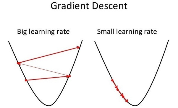
Repeating this process is what we refer to as training/fitting our model. We go through the whole training dataset, calculate our error values, and then calculuate the gradient. We then use the gradient to update the weight and bias values by a small amount. Training is complete when our error reaches an acceptable level or when it starts to converge.
Before training, we generally initialise our weight and bias to just random values.
Visualisation
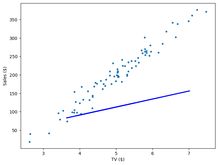
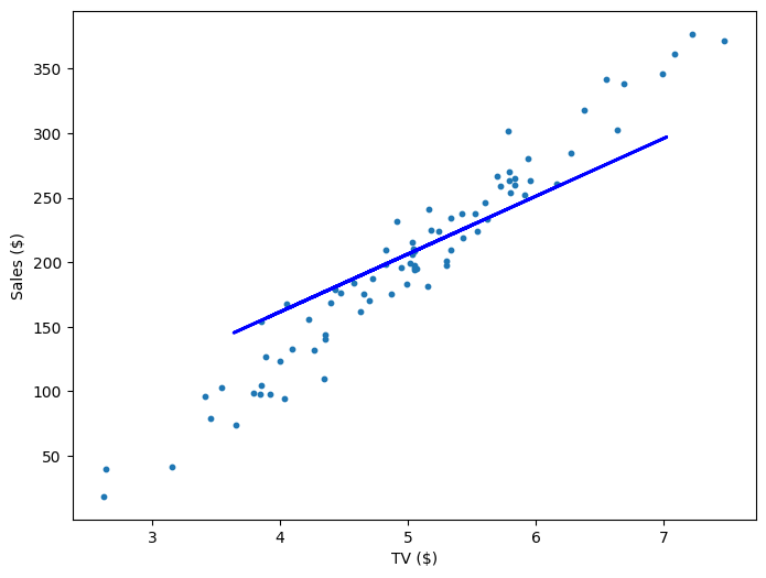
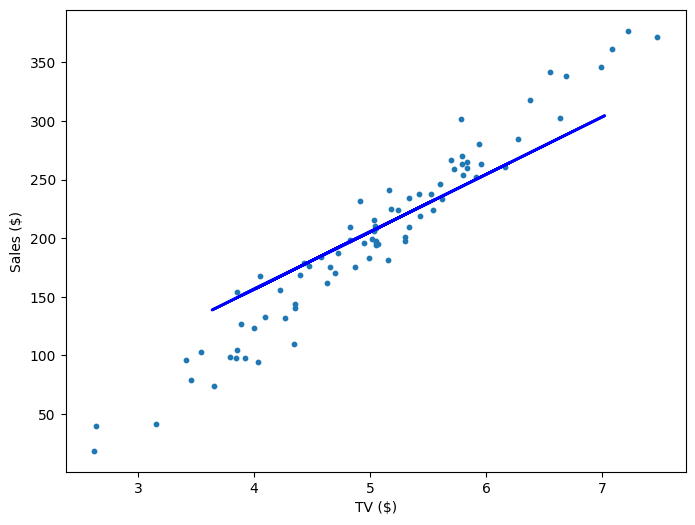
If our model is working, then as we fit it to our training data, we should see it's weight and bias changing as the loss decreases.
| Iteration | Weight | Bias | Loss |
|---|---|---|---|
| 0 | 21.71 | 4.02 | 10545.35 |
| 200 | 44.82 | -17.81 | 918.33 |
| 400 | 49.01 | -39.64 | 757.99 |
| 600 | 52.61 | -58.45 | 639.32 |
| 800 | 55.72 | -74.65 | 551.53 |
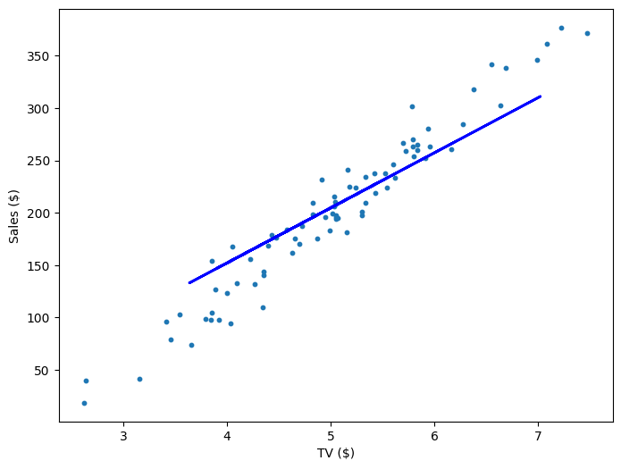
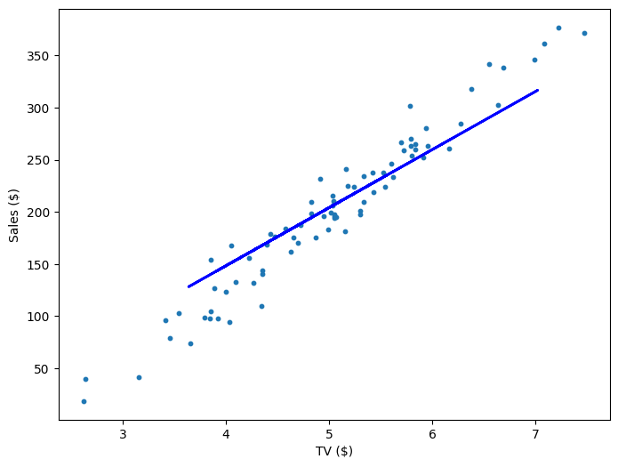
Multivariable Regression
Fortunately, the math doesn't actually get that much more complicated even as we add more variables (features). We just have to keep track of more partial derivatives, but the way we calculate those partial derivatives is the same! The trickiest thing actually is just keeping track of the notation. Here, \(x_j^i \) refers to the \(jth \) column and the \(ith \) row. In other words, it's the value of the \(jth \) variable for the \(ith \) data point. So, using all the columns in our table, our functions would just change accordingly:
\[ \text{Sales} = w_1 \text{Social Media} + w_2\text{TV} + w_3\text{Billboards} + b = w_1x_1 + w_2x_2 + w_3x_3 \]
\[ \mathcal{L}(w_1, w_2, w_3, b) = \frac{1}{N}\sum_{i=1}^{n}(y_i - (w_1 x_1^i + w_2 x_2^i + w_3 x_3^i + b))^2 \]
\[ \mathcal{L}' (w_1, w_2, w_3, b) = \begin{bmatrix} \frac{1}{N} \sum_{i=1}^{n} -2 x_1^i (y_i - (w_1 x_1^i + w_2 x_2^i + w_3 x_3^i + b)) \newline \frac{1}{N} \sum_{i=1}^{n} -2 x_2^i (y_i - (w_1 x_1^i + w_2 x_2^i + w_3 x_3^i + b)) \newline \frac{1}{N} \sum_{i=1}^{n} -2 x_3^i (y_i - (w_1 x_1^i + w_2 x_2^i + w_3 x_3^i + b)) \newline \frac{1}{N} \sum_{i=1}^{n} -2 (y_i - (w_1 x_1^i + w_2 x_2^i + w_3 x_3^i + b)) \end{bmatrix} \]
And that's it! Multivariable linear regression. You can see our functions get a little hard to parse though as we add more variables, so very often we'll simplify things with matrices. We construct a column vector \(\text{errors} = \text{targets} - \text{predictions}\), where the \(ith\) row is the result \(y_i - \hat{y_i}\), and we have an \(m \times n\) feature matrix \(X\) that contains our \(n\) data points for our \(m\) variables.
\[ \mathcal{L}' = \frac{-2}{N}X(\text{targets} - \text{predictions}) \]
So, for our example, if we had only 3 data points, the above equation might look like this:
\[ \mathcal{L}' = \frac{-2}{3} \begin{bmatrix} x_1^1 & x_1^2 & x_1^3 \newline x_2^1 & x_2^2 & x_2^3 \newline x_3^1 & x_3^2 & x_3^3 \newline 1 & 1 & 1 \newline \end{bmatrix} \begin{bmatrix} y_1 - \hat{y_1} \newline y_2 - \hat{y_2} \newline y_3 - \hat{y_3} \newline \end{bmatrix} \]
Notice that to account for \(b\), our feature matrix just has a row of ones. It's for that reason that very often we will just treat bias as a constant feature with weight \(w_0\).
Exercises
Your task is to implement a Linear Regression model. You must implement fit() which adjusts the weights and bias of your model to some training data and predict() which returns the predicted values of of an array of data points.
Inputs - fit():
Xis a NumPy NDArray (matrix) of data points such as[[1, 1, 0], [0, 0.5, 3], [0.7, 0.9, 0.3]], representing the training data (e.g., a set of coordinates [Social Media, TV, Billboards] for numerous companies).yis a NumPy NDArray (vector) of values such as[2, 3, 6], representing the corresponding values for each data point along an output axis (e.g., the sale revenue for each company).
Inputs - predict():
Xis a NumPy NDArray (matrix) of data points such as[[1, 1, 0], [0, 0.5, 3], [0.7, 0.9, 0.3]], representing a set of points we want to predict a continuous value for (e.g., a list of various company's advertising expenditure which we want to predict sales from)
Note: You would almost never calculate the gradient yourself in a production environment, but it's good to do it here just for understanding. When coding it up, you should be able to do it in just 1 line. Look at the final expression for \( \mathcal{L} \) for hints.
Extra Reading: Deterministic Linear Regressions
If you have ever taken a statistics or linear algebra class, you probably would have seen a very different way to perform a linear regression that didn't involve any gradient descent. Instead, it was probably one of the many deterministic algorithms for solving the least squares problem.
Remember that we're using gradient descent to try to find the right set of weights, \(w_1, ..., w_n\) and bias \(b\), such that that mean squared error \(\mathcal{L}\) is minimised. But is there a way we can find an exact solution for our weights and bias such that our loss is always minimised? The answer is yes! You can see a derivation here, but in short the optimal weights can be expressed as \(W = (X^T X)^{-1} X^T y\). If \(X\) is of full rank (independent data points >= features), then this means the optimal solution is unique. Otherwise, there exist many solutions, but we can use the pseudoinverse of \(X\) to find just one. There are other alternatives, but generally when you do a linear regression with Excel or some other statistical software, they are performing one of these algorithms.
So why should we use gradient descent? Well, for starters, the deterministic algorithms are slow. In most cases, a deterministic algorithm will take \(O(n^3)\) complexity, where \(n\) is the number of data points, mostly due to matrix inversion, calculating an SVD, or some other large matrix operation. In contrast, linear regression with gradient descent can take \(O(k n^2)\) complexity, where \(k\) is the number of iterations. When \(n\) is low (\(n < 10,000\)), the analytical solution might be better, but when Coles and Woolworths are frequently dealing with datasets of over 2 billion rows, it simply it isn't even a consideration. The analytical solutions can also prove more numerically unstable, meaning that errors which occur during the execution of the algorithm (like floating point rounding errors) can accumulate and significantly affect the result.
Extra Reading: Feature Scaling, Weight Initialisation, & Learning Rate
If you tried running your model on another toy dataset, you might have gotten a lot of NaN errors or your model simply took many more iterations to optimise. What you were most likely seeing was a smaller version of the vanishing/exploding gradients problem. Essentially, if your data deals with large values, the gradients are large, and your learning rate is high, you can end up taking such big steps that your predictions become increasingly worse/larger until they cannot be stored in even a 128 bit number. Alternatively, if your data deals with very small values, and your gradients are small (<1), then your step sizes will be accumulatively smaller and your weights will change very slowly.
To combat this, it's important to feature scale your data much like for KNN, and tune your learning rate with experimentation. It's also important that your weights are initialised with the right values (generally randomly between 0 and 1 is good).
Logistic Regression
What's the Problem?
The Academic Performance Team at your local university is trying to develop the perfect predictor for whether a student will pass or fail a unit based on various metrics they have access to. Because they've heard you're a talented (and cheap) data scientist, they've enlisted your help! You currently have access to a dataset like this
| Name | Hours Studied | Forum Engagement | Hours Doomscrolling | Pass/Fail |
|---|---|---|---|---|
| Michelle | 12.3 | 8.9 | 0.1 | P |
| John | 8.8 | 9.2 | 5.1 | P |
| Will | 6.5 | 2.1 | 2.0 | F |
| Colin | 9.4 | 0.3 | 3.1 | P |
| Bella | 2.2 | 0.1 | 14.3 | F |
Now, you already know K-Nearest Neighbours is a classification algorithm you could try using. However, there's likely some linear relationships in the data here (e.g., more hours studied = higher grade; more hours doomscrolling = lower grade). So, could we combine some of the techniques we learned for linear regression to create a pass/fail predictor?
What is a Logistic Regression
A logistic regression is a model that estimates the probability of an event as a linear combination of one or more variables. There's two types of logistic regression: binary (pass/fail) and multi (HD/D/C/P/F). To keep things simple, let's only focus on binary logistic regression for now.
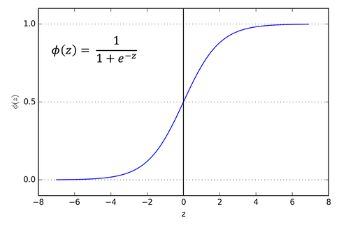
So, we have three features (Hours Studied, Forum Engagement, Hours Doomscrolling) and two classes (passed, failed). What we want is the output of a linear regression to somehow be a probability that the student passed. So, the output is any real value between 0 and 1, with 0 representing a fail and 1 a pass. To do this, we'll just feed the output of a regular linear regression into a sigmoid function:
\[ S: \mathbb{R }\to (0, 1), S(x) = \frac{1}{1 + e^{-x}} \]
\[ S(x) = \frac{1}{1 + e^{-(w_1\text{Hours Studied} + w_2\text{Forum Engagement} + w_3\text{Hours Doomscrolling} + b)}} \]
This maps any real value into a value between 0 and 1 and is what we often use in machine learning to map predictions to probabilities. It is an example of a logistic function. In machine learning, the raw inputs into this function are often called logits, but note that this is completely different from the mathematical definition 😖.
Making Predictions
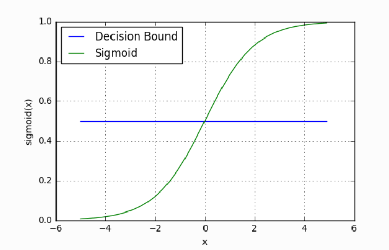
Our current model returns a probability score between 0 and 1, but we wanted it to map to a discrete class (Passed/Failed). To do this, we select a threshold value above which we classify a student as passed, and below which we classify a student as failed. For example, if our threshold was 0.5 and our probability was 0.2, we would classify the student as failed.
The nice thing is that we can tune this threshold to our liking depending on our usecase. For instance, for a preliminary medical screening for cancer, it might be a good idea to have a lower threshold because we'd rather have more false positives than miss a potential victim.
Loss Function & Training
Because all the parameters of our model are inside the linear regression function, we can just use the same training approach as we did for that model. That is, we'll use gradient descent to iteratively tune the weights and bias of our model.
Unfortunately, we shouldn't use the same loss function (Mean Squared Error) as we did for linear regression. Why? If you're inclined, there's a great written explanation by Michael Nielson on how the gradients decrease for increasingly worse predictions and a great video proof by Christian Nabert for it being non-convex. But, intuitively, MSE just doesn't punish our model enough for bad predictions.
Instead, we'll use Binary Cross-Entropy loss, also known as negative log loss.
\[ \mathcal{L} = \frac{-1}{N} \sum_{i=1}^{n}y_i\ln{(\hat{y_i})} + (1-y_i)\ln{(1-\hat{y_i})} \]
It might look a little confusing, but it's actually a very intuitive cost function. We can break it up into 2 cases, when our actual label (\(y_i\)) is 1 and when it's 0.
\[ \mathcal{L} = \ln{(\hat{y_i})} \hspace{2.6cm} \text{if y = 1} \]
\[ \mathcal{L} = \ln{(1 - \hat{y_i})} \hspace{2cm} \text{if y = 0} \]
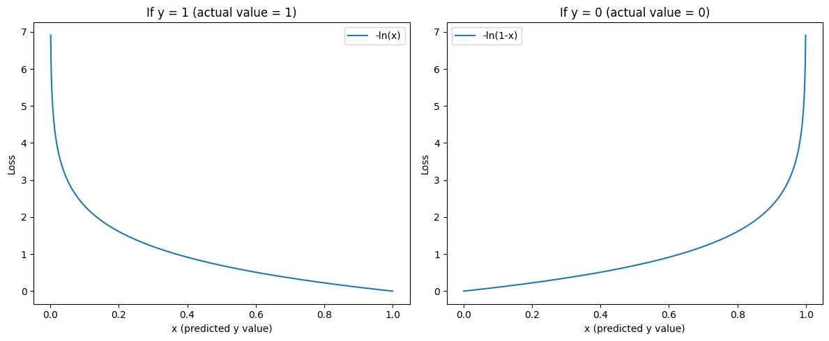
As you can see, our loss function is minimal when the prediction is correct, and it heavily penalises incorrect predictions.
Multiplying by \(y\) and \((1-y)\) in the general equation is just a neat way of combining the two functions into one equation, and just like MSE loss we take the average loss for all data points in our training dataset.
Gradient Descent
One of the really neat things about Binary Cross-Entropy loss is that the expression for its gradients with respect to the weights and bias are quite simple. I won't cover them here since they're a bit involved, but Nielson covers them and so does this stackexchange (note: the author does not take the mean of the loss here like we do).
\[ \mathcal{L}' (w, b) = \begin{bmatrix} \frac{\partial \mathcal{L}}{\partial w} \newline \frac{\partial \mathcal{L}}{\partial b} \end{bmatrix} = \begin{bmatrix} \frac{1}{N} \sum_{i=1}^{n} x_i(\hat{y_i} - y_i) \newline \frac{1}{N} \sum_{i=1}^{n} (\hat{y_i} - y_i) \end{bmatrix} \]
Exercise
Your task is to implement a Logistic Regression model. You must implement _sigmoid() which applies the sigmoid function piecewise to a vector, fit() which adjusts the weights and bias of your model to some training data, predict() which returns the predicted values of of an array of data points.
Inputs - _sigmoid():
xis a NumPy NDArray (vector) of values such as[1, 2, 3, 4], to which you should apply the sigmoid function in a piecewise fashion, returning, for example,[0.73105858 0.88079708 0.95257413 0.98201379].
Inputs - fit():
Xis a NumPy NDArray (matrix) of data points such as[[1, 1, 0], [0, 0.5, 3], [0.7, 0.9, 0.3]], representing the training data (e.g., a set of coordinates [Hours studied, Forum engagement, Hours doomscrolling] for numerous students).yis a NumPy NDArray (vector) of values such as[0, 1, 0], representing the corresponding binary class for each data point (e.g., whether the student has passed or failed the unit).
Inputs - predict():
Xis a NumPy NDArray (matrix) of data points such as[[1, 1, 0], [0, 0.5, 3], [0.7, 0.9, 0.3]], representing a set of points we want to predict a binary class for (e.g., a list of various students' metrics from which we want to predict whether they pass or fail).
Bonus: You might notice that there is a lot of repeated code between your Linear Regression and Logistic Regression classes. While I might think that's fine, an OOP purist would promptly send you to the gallows. So, see if you can try to combine some of the functionality into a parent class or abstract class.
Softmax Regression
What's the Problem?
The Academic Performance Team at your local university would like to extend the pass/fail predictor you made to predict the grade the student will receive (HD/D/C/P/F).
| Name | Hours Studied | Forum Engagement | Hours Doomscrolling | Grade |
|---|---|---|---|---|
| Michelle | 12.3 | 8.9 | 0.1 | HD |
| John | 8.8 | 9.2 | 5.1 | D |
| Will | 6.5 | 2.1 | 2.0 | F |
| Colin | 9.4 | 0.3 | 3.1 | C |
| Bella | 2.2 | 0.1 | 14.3 | F |
Is there some way you could extend the binary logistic regression classifier you made earlier to support multiple classes?
What is a Softmax Regression
A softmax regression is a generalisation of the logistic regression which supports the estimation of the probabilitity of multiple events. Luckily not much changes between the two models, but there are some key differences.
Firstly, because we're calculating the probability of multiple classes, we now need to provide logits for each class. So, for each data point we pass into the linear part of our model, we should return a vector like this, with a row for each class.
\[ \textbf{z} = \begin{bmatrix} 1.3 \newline 5.1 \newline 2.2 \newline 0.7 \newline 1.1 \newline \end{bmatrix} \in \mathbb{R} \]
This means that our weights matrix, $W$, needs to be extended. So instead of just being \(\text{features} \times 1\) like it was for logistic regression, it now needs to be \(\text{features} \times \text{classes}\). Similarly, our bias, \(b\), should go from \(1 \times 1\) to a \(\text{classes} \times 1\) matrix too.
Additionally, to convert these logits to probabilities we also generalise the sigmoid function to the softmax function.
\[ \sigma(\textbf{z})_i = \frac{e^{z_i}}{\sum_{j=1}^{K}e^{z_j}} \]
- \(\sigma_i\) = value for the $ith$ row of the softmax output vector
- \(\textbf{z}\) = input vector
- \(e^{z_i}\) = exponential for the $ith$ row of the input vector
- \(e^{z_j}\) = exponential for the $jth$ row of the input vector. We sum these up for each row of the input vector.
Passing the above logits into this thus gives us a vector with the probability that the data point belongs to each class.
\[ \sigma(\textbf{z}) = \begin{bmatrix} 0.02 \newline 0.90 \newline 0.05 \newline 0.01 \newline 0.02 \newline \end{bmatrix} \]
Since all of these terms add up to 1, instead of having a decision boundary, we predict which class a data point belongs to by picking the row with the highest value. So in this case, \(\textbf{z}\) belongs to class 1 (row 2), which has a probability of 0.90. This operation is what's often called taking the \(\text{argmax}\) of \(\textbf{z}\).
A very nice summary of all this by Sophia Yang is included below:
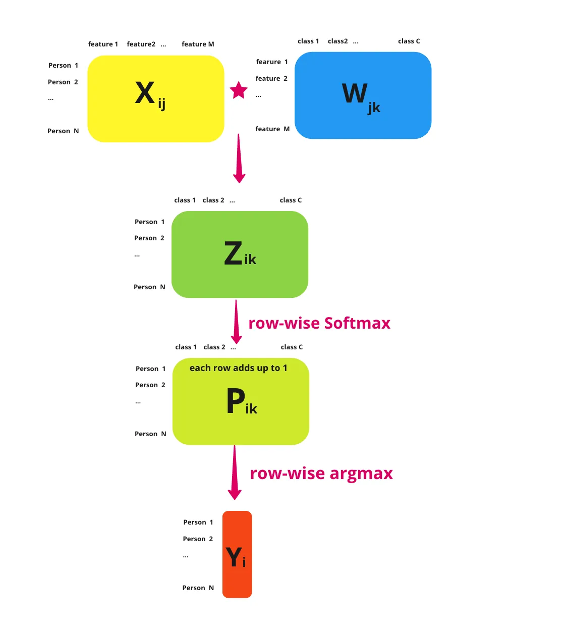
Loss Function & Training
Likewise, we need to adjust the way we train our model. Firstly, because we're dealing with multiple classes, most datasets will just simply add the extra classes to their target vector, \(\textbf{y}\).
\[ \textbf{y} = \underset{\text{N targets for N data points}}{\underbrace{\begin{bmatrix} \vdots \newline 0 \newline 1 \newline 1 \newline 2 \newline 3 \newline \vdots \end{bmatrix}}} \]
However, because we want to correct our model for each wrong probability per class, to make things easier we create a one-hot encoding. That is, if we have \(N\) data points and \(K\) classes, we create an \(N \times K\) matrix, \(Y\), where \(Y_{i, j}\) is 0 if the \(ith\) data point is not the \(jth\) class and 1 if it is. So for the above vector,
\[ Y = \begin{bmatrix} \vdots & \vdots & \vdots & \vdots \newline 1 & 0 & 0 & 0 \newline 0 & 1 & 0 & 0 \newline 0 & 1 & 0 & 0 \newline 0 & 0 & 1 & 0 \newline 0 & 0 & 0 & 1 \newline \vdots & \vdots & \vdots & \vdots \end{bmatrix} \]
We also generalise the binary cross entropy loss function to just the cross entropy loss functions
\[ \mathcal{L} = \frac{-1}{N}\sum_{i=1}^{n} \sum_{j=1}^{K} y_{i, j} \ln(\hat{y}_{i, j}) \]
- \(y_{i, j} \in {0, 1}\) = True label for the \(ith\) data point for the \(jth\) class
- \(\hat{y}_{i, j} \in \mathbb{R}\) = Predicted probability for the \(ith\) data point for the \(jth\) class.
The really nice thing though is that this doesn't change our gradient expression at all.
\[ \mathcal{L}' (w, b) = \begin{bmatrix} \frac{\partial \mathcal{L}}{\partial w} \newline \frac{\partial \mathcal{L}}{\partial b} \end{bmatrix} = \begin{bmatrix} \frac{1}{N} \sum_{i=1}^{n} x_i(\hat{y_i} - y_i) \newline \frac{1}{N} \sum_{i=1}^{n} (\hat{y_i} - y_i) \end{bmatrix} \]
Exercise
Your task is to implement a Softmax Regression model. You must implement fit() which adjusts the weights and bias of your model to some training data, predict() which returns the predicted classes of of an array of data points.
Inputs - fit():
Xis a NumPy NDArray (matrix) of data points such as[[1, 1, 0], [0, 0.5, 3], [0.7, 0.9, 0.3]], representing the training data (e.g., a set of coordinates [Hours studied, Forum engagement, Hours doomscrolling] for numerous students).yis a NumPy NDArray (vector) of values such as[0, 1, 2], representing the corresponding class for each data point (e.g., what grade the student received). You can assume that all class labels will appear here and that they are continuous natural numbers.
Inputs - predict():
Xis a NumPy NDArray (matrix) of data points such as[[1, 1, 0], [0, 0.5, 3], [0.7, 0.9, 0.3]], representing a set of points we want to predict a class for (e.g., a list of various students' metrics from which we want to predict their grade).
Perceptron
It’s Nothing New!
So far, you’ve actually come across all the ingredients for building a neural network: linear regression, loss functions, gradient descent, activation functions. But, if you went ahead and read a Deep Learning paper, you’d probably find yourself unfamiliar with a lot of the terminology. This is mostly because the field has a lot of its own vocabulary and they tend to misuse and relabel their own terms and terms from other branches of mathematics. So, in this article we’re going to cover some history and revisit all of these concepts but in the context of the “perceptron”, the core unit of neural networks. In doing so, hopefully you’ll be less confused in future and will have a greater appreciation for the field’s history.
The McCulloch-Pitts Model
The initial model for the perceptron dates back to Warren McCulloch (neuroscientist) and Walter Pitts (logician) in 1943. They described biological neurons as subunits of a neural network in the brain. Signals of variable magnitude arrive at the dendrites, they accumulate in the cell body, and if they exceed a certain threshold, they pass onto the next neuron.
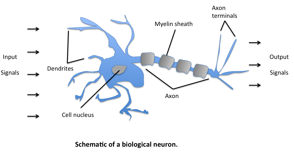
The two scientists simplified this into a Boolean model called a perceptron, something which takes in a bunch of True/False values, counts them, and returns True/False depending on if the count meets some threshold.
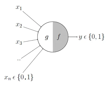
For instance, here \(g\) takes in the input Booleans \(x_1, …, x_n\), aggregates them, and then \(f\) decides whether to output a True or False.
So, for example
- \(x_1\) could be the question "Have I Eaten?"
- \(x_2\) could be "Is it Evening?"
- \(x_3\) could be "Is that girl texting me?"
- \(x_4\) could be "Is work due tomorrow?"
And \(y\) could be the result "Will I be happy tonight?". \(f\) then might specify that if at least 3 of these are true, then \(y\) is true. More formerly, we'd express the model like this where \(\theta\) is our activation threshold (3):
\[ g(x_1, x_2, x_3, ..., x_n) = g(\textbf{x}) = \sum_{i=1}^{n} x_i \]
\[ y = f(g(\textbf{x})) = \begin{cases} 1 & \text{if } g(\textbf{x}) \geq \theta \newline 0 & \text{otherwise} \end{cases} \]
McCulloch and Pitts demonstrated that this model could be used to represent AND, OR, NOT, NAND, and NOR gates, and they also showed that they admit a nice geometric interpretation. If we draw up the input variables \(x_1, ..., x_n\) on their own axes, then our \(\theta\) value admits a decision boundary in the space.
So, for 2 input variables there are only 4 possible combinations for the input - (0, 0), (0, 1), (1, 0), (1, 1). If we set \(\theta = 1\), then we effectively create an OR gate, and geometrically, our perceptron will return 1 if our input lies above the decision boundary, and 0 if it lies below.
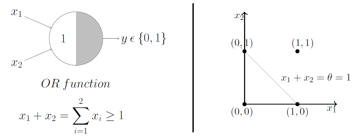
What do you think will happen if we change the \(\theta\) value?
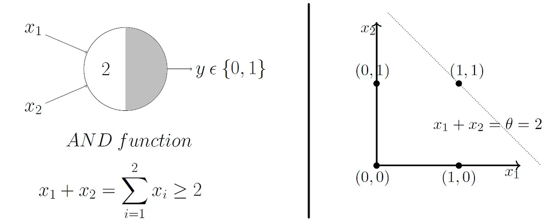
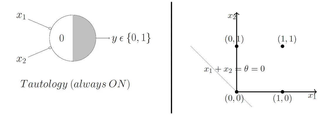
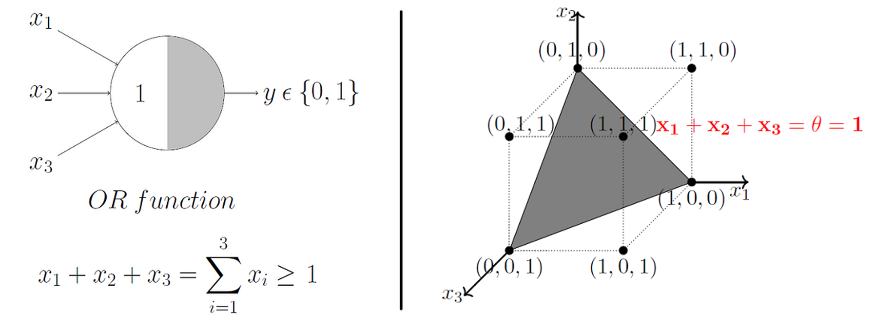
Beautifully, this model extends to higher dimensions just as easily. So, in 3D, our decision boundary just becomes a plane instead of a line.
The Rosenblatt Artificial Neuron
Some big problems with the McCulloch-Pitts model are that it required us to handcode the \(\theta\) threshold and that all of our inputs contributed to the result equally. In 1957 Frank Rosenblatt would solve these by introducing the idea of learnable weights.
Instead of restricting our inputs to boolean variables, we'd allow any real number and just multiply each by a weight parameter. We'd aggregrate these products like in the McCulloch-Pitts model and only return a 0 or 1 depending on if it meets a certain threshold.
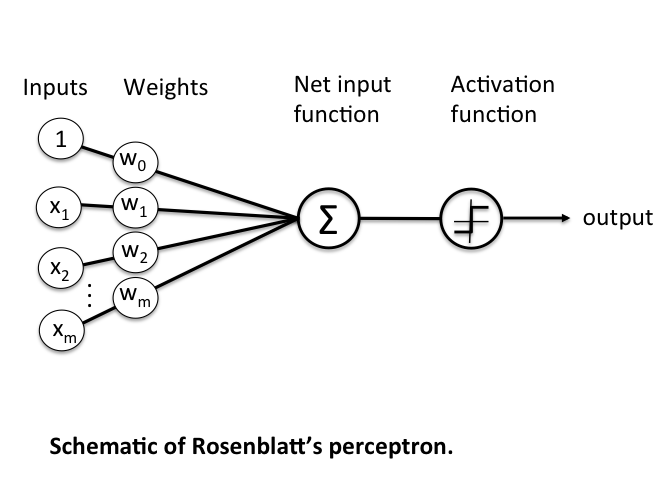
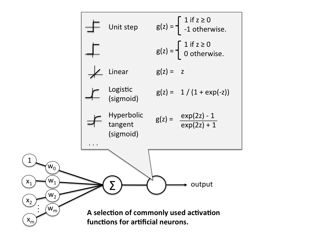
More formerly, we define \(\textbf{z}\) to be the linear combination of input values \(\textbf{x}\) and weights \(\textbf{w}\), which we pass through an activation function \(g(\textbf{z})\) that enforces our threshold.
Mathematically, \(g(\textbf{z})\) is the "unit step function" or "heaviside step function" and can be defined as
\[ g(\textbf{z}) = \begin{cases} 1 & \text{if } \textbf{z} \geq \theta \newline 0 & \text{otherwise} \end{cases} \]
where
\[ \textbf{z} = x_1 w_1 + ... + x_n w_n = \sum_{i=1}^{n} x_i w_i = \textbf{x}^T \textbf{w} \]
\(\textbf{w}\) is the weight vector, and \(\textbf{x}\) is an \(n\)-dimensional sample from some training data.
\[ \textbf{x} = \begin{bmatrix} x_1 \newline \vdots \newline x_n \end{bmatrix} \quad \textbf{w} = \begin{bmatrix} w_1 \newline \vdots \newline w_n \end{bmatrix} \]
The problem is that we still have a \(\theta\) value we need to hardcode. To fix that, we just need to realise that having a \(\theta\) threshold is just the same as adding \(\theta\) to our linear combination, adding a bias to our result. We can then just treat this as another weight we need to learn, \(w_0\), with a constant input of \(x_0 = 1\). This simplifies our activation function to
\[ g(\textbf{z}) = \begin{cases} 1 & \text{if } \textbf{z} \geq 0 \newline 0 & \text{otherwise} \end{cases} \]
Rosenblatt's Learning Model
The learning rules for Rosenblatt's artifical neuron are actually quite simple.
- Initialise the weights to small random numbers
- For each training sample \(\textbf{x}^i\):
- Calculate the output, \(\hat{y_i}\)
- Update all the weights.
The output \(\hat{y_i}\) is the True/False value (class label) from earlier (0 or 1), and each weight update can be written formerly as
\[ w_j := w_j + \alpha \Delta w_j \]
where \(\alpha\) is the learning rate, a value in \([0, 1]\)
The value for calculating \(\Delta w_j\) is also quite simple
\[ \Delta w_j = x_j^i(y_i - \hat{y_i}) \]
- \(w_j\) = the \(jth\) weight parameter
- \(x_j^i\) = the \(jth\) value of the \(ith\) \(\textbf{x}\) vector in our training dataset.
- \(y_i\) = the actual class label (0 or 1) for the \(ith\) training point.
- \(\hat{y_i}\) = the predicted class label (0 or 1) for the $ith$ training point.
Although the notation might seem a bit awful, the logic behind this rule really is quite beautifully simple. Let's have a look at what possible values we might get.
\[ \begin{matrix} y_i & \hat{y_i} & y_i - \hat{y_i} \newline 1 & 1 & 0 \newline 1 & 0 & 1 \newline 0 & 0 & 0 \newline 0 & 1 & -1 \newline \end{matrix} \]
We can see that the weights are pushed towards negative or positive target classes depending on how the prediction is wrong! By multiplying this with \(x_j^i\), we change weights proportionally to how much they affected the end result.
Again, it's important to note that we update all the weights per training sample. A complete run over all the training samples is called an epoch. We can then train for an arbitrary amount of epochs or until we reach some accuracy.
Adapative Linear Neuron (ADALINE)
A problem with Rosenblatt's model though is that it doesn't account for how wrong the model's predictions are when updating the weights. To account for that, in 1960 Bernard Widrow and Tedd Hoff created the Adaptive Linear Neuron (ADALINE).
In contrast to the Rosenblatt model, the activation function is just the identity function (do nothing), and only when we need to make a prediction do we put it into the unit step function (quantizer). NOTE: often the identity function will be referred to as a "linear activation function", since the aggregator is a linear combination of inputs.
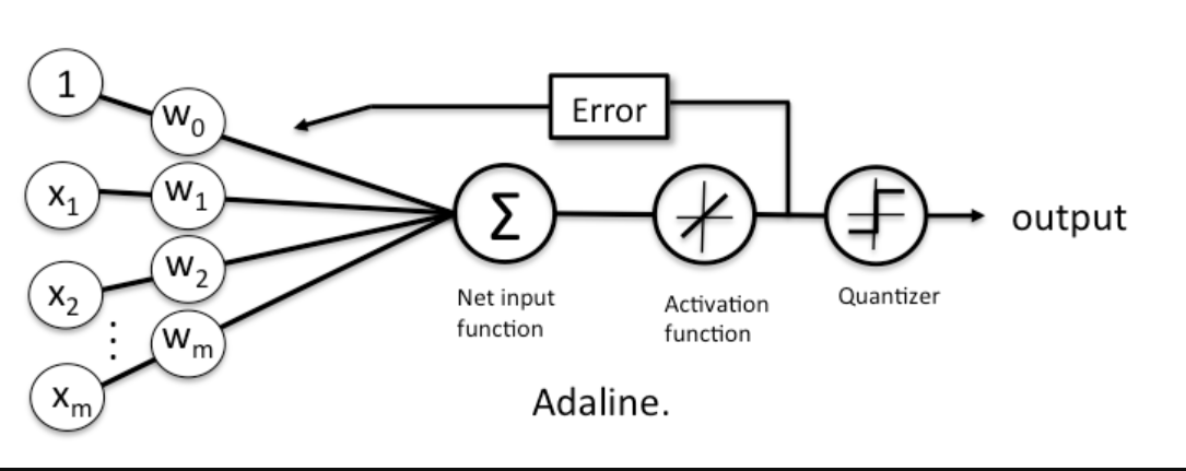
While this might seem like a step back, the big advantage of the linear activation function is that it's differentiable, so we can define a loss/cost function, \(\mathcal{L}(\textbf{w})\) that we can minimise to update our weights. In this case, we'll define our loss function to be the mean squared error.
\[ \mathcal{L}(\textbf{w}) = \frac{1}{n}\sum_{i=1}^{n}(y_i - \hat{y_i})^2 \]
We can minimise this loss function using gradient descent, giving us a new update rule for our weights.
\[ \mathcal{L}' = \frac{-2}{n} X (\textbf{y} - \hat{\textbf{y}}) \]
\[ \textbf{w} := \textbf{w} + \alpha \Delta \textbf{w} \]
There are 2 key differences to the Rosenblatt model that you should notice here
- \(\hat{\textbf{y}}\) is a vector of real numbers, not class labels. These are the raw predictions that come from the linear combination of weights. Often these will be called "logits". Because these can vary a lot in magnitude, it's important to apply feature scaling in your model.
- The weights are updated based on all samples in the training set at once (instead of updating incrementally after each sample).
Non-Linear Activation Functions
The remaining problem with ADALINE is that it was still effectively just separating some space with a linear decision boundary. Even if we combined multiple perceptrons together, it could still be simplified down to just one single neuron and one single decision boundary. Not all data, however, can be separated with just a straight line, plane, or hyperplane.
In 1989 this was solved by George Cybenko, who demonstrated that we can model non-linear datasets by setting our activation function to the sigmoid function:
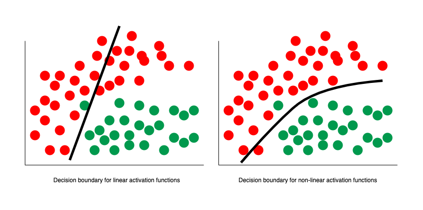
In fact, Cybenko demonstrated something much stronger than that. He showed that if we combined such neurons into a "neural network" (with even just one layer), then we could approximate any continuous function to any desired precision.
So, I could give you any function, like some random squiggle:
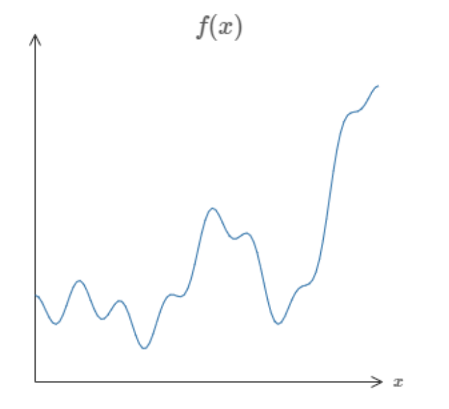
And there is guaranteed to exist a network of neurons that could could approximate this function to some arbitrary precision.
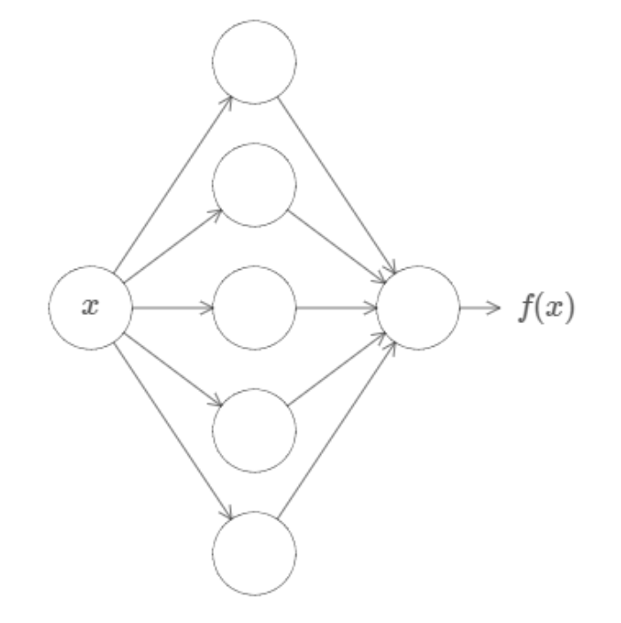
While that might not make a lot of sense now, this is a profound result and is the first of the Universal Approximation Theorems, which underpin a lot of the theory behind deep learning today. You can find links to the official proofs on the Wikipedia page (even for other activation functions!) but if you want just an intuition for the proof, I highly reccommend either this video or article by Nielsen.
The main thing to know is that this is essentially the modern blueprint for the artifical neuron which makes up the neural networks which power so much of AI today. Although there is technically a distinction between "perceptron" and "artifical neuron", most people will just use both terms to refer to this.
Exercise
Your task is to implement the Rosenblatt perceptron. You must implement fit() which adjusts the weights and bias of your model to some training data an predict() which returns the predicted values of of an array of data points.
Inputs - fit():
Xis a NumPy NDArray (matrix) of data points such as[[1, 1, 0], [0, 0.5, 3], [0.7, 0.9, 0.3]], representing the training data.yis a NumPy NDArray (vector) of values such as[0, 1, 0], representing the corresponding binary class for each data point.
Inputs - predict():
Xis a NumPy NDArray (matrix) of data points such as[[1, 1, 0], [0, 0.5, 3], [0.7, 0.9, 0.3]], representing a set of points we want to predict a binary class for. So, you should return a NumPy NDArray (vector) like[0, 0, 1].
Note: The Rosenblatt Perceptron is pretty much found nowhere today, but it's still a good exercise to implement, and you should see a lot of similarities between this and your implementations of Linear Regression and Logistic Regression.
Why Don't We Just Study Deep Learning Now?
Great! You've just learned the core unit for neural networks. You might be wondering why we don't just dive right in and study neural networks and deep learning now. Especially with all the hype around LLMs and GNNs, it can seem like classical ML algorithms are ancient and obsolete.
However, this couldn't be further from the truth. In fact, classical ML is still used extensively and here are just some of the advantages:
- Explainability: Neural Networks can be near impossible to justify, because often the values for weights and biases don't correspond to any logic we'd understand. Conversely, classical ML models are easy to visualise and have human explainable parameters.
- Speed: While in theory neural networks can approximate any function, they often need a lot of perceptrons and, by extension, a lot of parameters to do so. Because of that, they can take a long time to train and can be too memory intensive to even run on some devices. Conversely, classical ML algorithms are generally more efficient and boast plenty of room for optimisation (especially with easy parallelisation!).
- Superior Performance: On some datasets, classical ML algorithms can perform the same or even better than most deep learning techniques. There's a great paper demonstrating this with a good summary on Medium
So, whenever you need to solve a new problem here's the thought process you should take:
- Is there a deterministic algorithm I can use to solve this?
- Could I use some classical ML algorithms to help me solve this?
- Did I really consider all my options?
- sigh, how can I use Deep Learning to help me solve this?
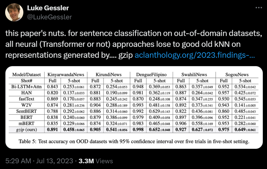
I'll end with this Tweet which depicts how this paper from 2023 demonstrated that KNN - yes, the very first algorithm you learnt! - outperformed deep neueral networks with millions of parameters.
Extra Reading: Variants of Gradient Descent
One of the important differences for ADALINE compared to the Rosenblatt model was that it updated the weights based on all training samples at once, rather than updating them incrementally for each sample. In formal terms, we describe ADALINE's learning method as vanilla gradient descent. In contrast, since the parameters of the Rosenblatt model change more frequently, we call it stochastic gradient descent.
There are positives and negatives to both of these methods. For instance, vanilla gradient descent guarantees convergence to some local minimum of the loss function, but it is usually slow and painful. Stochastic gradient descent performs more frequent updates so it can often converge fasters, but it can also result in more oscillations.
A nice compromise between the both of these is mini-batch gradient descent, which updates the parameters of your model after seeing a set amount of training samples (a batch).
But there are plenty more variants of gradient descent, and we call each of these algorithms "optimisers". Often, you'll see Adam and SGD being used in most deep learning projects, because they empirically perform the best on the widest range of data. But if you want a really good comparison between current optimisers, I highly reccommend this review paper.
Note: People will often use SGD (stochastic gradient descent) to describe vanilla gradient descent, mini-batch gradient descent, and many other variants which introduce momentum. While admittedly a bad trend, it's made its way into most machine learning libraries, so we'll often use these terms interchangeably too from here on out.
Naive Bayes Classifier
What's the Problem?
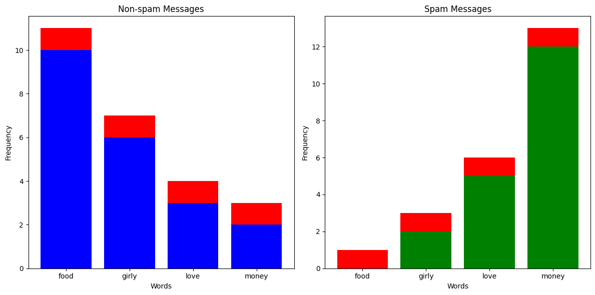
You've been getting a lot more spam bots texting you lately, and instead of blocking them manually, you've decided to build a classifier which can automatically predict whether a message is spam or not. You've noticed that messages from spam bots tend to have different vocabulary compared to what your friends send you, so you take a sample of messages and plot how many times certain words appear.
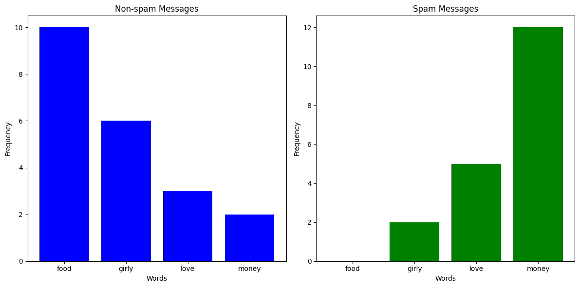
Clearly, if some words appear more than others, it is more likely that the message is from a spam bot. So, could we build a probabilistic classifier around that?
What is a Naive Bayes Classifier?
The idea behind Naives Bayes Classifiers is actually quite simple. Let's say we had \(K\) classes and \(n\) features, then if we assigned probabilities \(p(C_k | x_1, ..., x_n)\) to each class \(C_k\) given we have some feature vector \(\textbf{x} = (x_1, ..., x_n)\), then the model's best prediction would just be the class with the highest probablitiy.
For example, let's say we got a text with 4 occurences of the word "food", 2 occurences of the word "girly", 6 occurences of the word "love", and 0 occurrences of the word "money". We could represent that text as a vector \(\textbf{x} = (4, 2, 6, 0)\). Now, let's say that \(p(\text{Spam Message} | \textbf{x}) = 0.19\) and \(p(\text{Non-spam Message} | \textbf{x}) = 0.6\), then we would confidently say that the message is not spam.
The problem is how do we work out \(p(C_k | \textbf{x})\)? Fortunately, Bayes' Theorem comes to the rescue, because it tells us the conditional probabilitiy can be expressed as
\[ p(C_k | \textbf{x}) = \frac{p(C_k) p(\textbf{x} | C_k)}{p(\textbf{x})} \]
Often in Bayesian probability, the above equation will also be phrased as follows
\[ \text{posterior} = \frac{\text{prior} \times \text{likelihood}}{\text{evidence}} \]
We notice that for all \(C_k\), the denominator \(p(\textbf{x})\) doesn't change, so it's effectively a constant. Since we don't really care about the actual probability values but rather the predictions, we can just get rid of it for now to simplify our equations.
\[ p(C_k | \textbf{x}) \propto p(C_k) p(\textbf{x} | C_k) \]
\(\propto\) is the "proportional to" symbol, since strictly speaking the terms aren't equal
Now, by using the chain rule repeatedly and by assuming that each of the features of \(\textbf{x}\) are independent (see here for details), we can get the following expression
\[ p(C_k | \textbf{x}) \propto p(C_k)\prod_{i=1}^{n}p(x_i|C_k) \]
That means, with some feature vector \(\textbf{x}\), our prediction \(\hat{y}\) will be
\[ \hat{y} = \underset{k \in \{0, ..., K\}}{\text{argmax}} p(C_k)\prod_{i=1}^{n}p(x_i|C_k) \]
Sometimes, however, some probabilities will be so small that the actual numbers risk underflowing on a computer, causing weird undefined behaviour. For that reason, some models will just take the log probability of everything.
\[ \hat{y} = \underset{k \in \{ 0, ..., K \}}{\text{argmax}} \log{(p(C_k))} + \sum_{i=1}^{n} \log{(p(x_i|C_k))} \]
Types of Naive Bayes Classifier
There are many different types of Naive Bayes Classifiers depending on what sort of probability distributions the feature variables are sampled from.
- Bernoulli Naive Bayes: This is used with vectors with Boolean variables, such as \(\textbf{x} = (1, 1, 0, 0, 1)\).
- Multinomial Naive Bayes: This is used with features from multinomial distributions. This is especially useful for non-negative discrete data, such as frequency counts. The above examples of counting words in a text message are a good example of this. Here, if the probability of seeing the word in a text message given a certain class is \(p_k\), the likelihood of it appearing \(c\) times would be \(p_k^c\).
- Gaussian Naive Bayes: This is used with Gaussian/normal distributions. Typically when our feature variables are continuous, we assume that they're sampled from a gaussian distribution, and we thus calculate the likelihood \(p(x_i | C_k)\) as follows
\[ p(x_i | C_k) = \frac{1}{\sqrt{2 \pi \sigma_k^2}}e^{-\frac{(x_i - \mu_k)^2}{2 \sigma_k^2}} \]
- \(\sigma_k^2\) is the variance of \(x_i\) associated with the class \(C_k\)
- \(\mu_k\) is the mean of \(x_i\) associated with the class \(C_k\)
Alpha Value
Let's say you've received a text message with 20 occurrences of the word "money" and 1 occurrence of the word "food". Just looking at the column chart above, you'd expect that the text message would be labelled as spam. But since there aren't any spam messages in the training data with the word "food", the likelihood of having 1 occurrence in a spam message is 0, meaning \(p(\text{Spam Message} | (1, 0, 0, 20)) = 0\). This is clearly a problem, so what we do is something called Laplace smoothing. Effectively, we add an \(\alpha\) to all the occurences of everything in our training set to avoid multiplying anything by 0.
Exercise
Multinomial Classifier
Your task is to implement a Multinomial Naive Bayes Classifier. You must implement fit() which takes training data and preprocesses it for predictions, and _predict() which returns the predicted class for a given feature vector. You should account for an \(\alpha\) value, but you should not use \(\log\) probabilities.
Inputs - fit():
Xis a NumPy NDArray (matrix) of feature vectors sampled from a multinomial distribution that form your training data. For example,[[1, 1, 0, 1], [2, 3, 4, 1], [3, 4, 2, 1]]. In context of the spam filter, you could imagine each inner as a counter for a text message, with each number representing the occurences of a certain word.yis a NumPy NDArray (vector) representing the classes of each feature vector ofX. For example,[0, 0, 1]. In context of the spam filter, you could imagine each number corresponding to a True/False of whether each corresponding text message is spam.alphais a non-negative integer representing the Laplace smoothing parameter. This represents how much you should add to each feature count per class for calculating likelihood.
Inputs - _predict():
xis a NumPy NDArray (vector) representing a feature vector sampled from a multinomial distribution which you should predict the class of from the training data. For example,[1, 2, 0, 1].
Gaussian Classifier
Your task is to implement a Gaussian Naive Bayes Classifier. You must implement fit() which takes training data and preprocesses it for predictions, and _predict() which returns the predicted class for a given feature vector. You do not need to account for an \(\alpha\) value, but you should use \(\log\) probabilities.
Inputs - fit():
Xis a NumPy NDArray (matrix) of feature vectors with continuous values that form your training data. For example,[[23.4, 11.2, 1.2], [4.3, 5.6, 1.2], [3.3, 2.2, 14.2]]. For some context, you could imagine each inner array as some summary of a customer, and each value as the average number of minutes spent in certain stores.yis a NumPy NDArray (vector) representing the classes of each feature vector ofX. For example,[2, 0, 1]. In the same context, these labels could refer to whether the customer is "non-binary, male, female".
Inputs - _predict():
xis a NumPy NDArray (vector) representing a feature vector with continuous values which you should predict the class of from the training data. For example,[1.2, 1.1, 6.3].
Extra Reading: What is so naive?
Remember that at the basic level, a Naive Bayes Classifier wants to find the \(p(C_k | \textbf{X})\) with the greatest value. To calculate this, it needs to calculate \(p(\textbf{x} | C_k)\). However, because this value is generally hard to calculate, we make a big assumption that the features of \(\textbf{x}\) are independent, so we can end up with the formula \(p(\textbf{x} | C_k) = p(x_1 | C_k) \times p(x_2 | C_k) \times p(x_3 | C_k) \times \dots\). It's this assumption that we call naive, because it may or may not turn out to be correct.
There is actually a fantastic intuitive explanation of this on Wikipedia
All naive Bayes classifiers assume that the value of a particular feature is independent of the value of any other feature, given the class variable. For example, a fruit may be considered to be an apple if it is red, round, and about 10 cm in diameter. A naive Bayes classifier considers each of these features to contribute independently to the probability that this fruit is an apple, regardless of any possible correlations between the color, roundness, and diameter features.
Of course, very often this assumption is incorrect, but even in those cases, Naive Bayes Classifiers can still perform remarkably well. In fact, they can even outperform models that don't make such an assumption because they can avoid some of the pitfalls of the curse of dimensionality. For example, if two features are dependent, such as hair length and gender, then assuming independence lets you double count the evidence, which is especially helpful when you're dealing with many, many features.
A more mathematical explanation for Naive Bayes effectiveness can be found in research, but the explanations get quite a bit more involved.
Support Vector Machine (SVM)
Revisiting Classification
Let's recall the problem of binary classification that we saw for the perceptron. Remember that what we essentially wanted before our activation function was some function like this
$ f(\bold{x_i}) = \begin{cases} \geq 0 & \text{if } y_i = 1 \ < 0 & \text{if } y_i = 0 \end{cases} $
Where the output is positive for our data point $\bold{x_i}$, if the corresponding $ith$ class label is $1$, and negative if the class label is $0$.
Note, for now, we're going to set our class labels to $1$ and $-1$. This is because we can then cleverly characterise a correct prediction as $y_i f(\bold{x_i}) > 0$.
Anyways, the way we achieved that was by setting $f$ to some linear function like $f(\bold{x_i}) = \bold{x_i} \bold{w} + b$. We also briefly mentioned that this function has a geometric interpretation. Namely, $f(\bold{x}) = 0$ represents a hyperplane dividing our two classes.
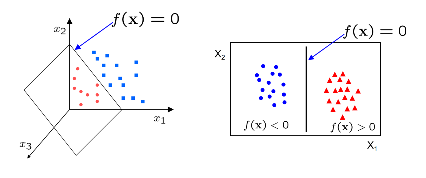
Eventually, we ended up training our weights by defining a loss function $\mathcal{L}$, which we performed gradient descent against. The loss function we used was mean-squared error. While this was good, MSE did not put particular emphasis on how the optimal weights may generalise for unseen data. While it does try to create a sizeable gap between classes, the way it behaves is often hard to explain and extremely sensitive to pertubations in data.
For instance, while the top left of these obviously gives a high loss value, the rest all would provide "small enough" loss values for most people to assume training is complete. However, only the bottom right gives the most space to both classes to expand as needed for unseen data.
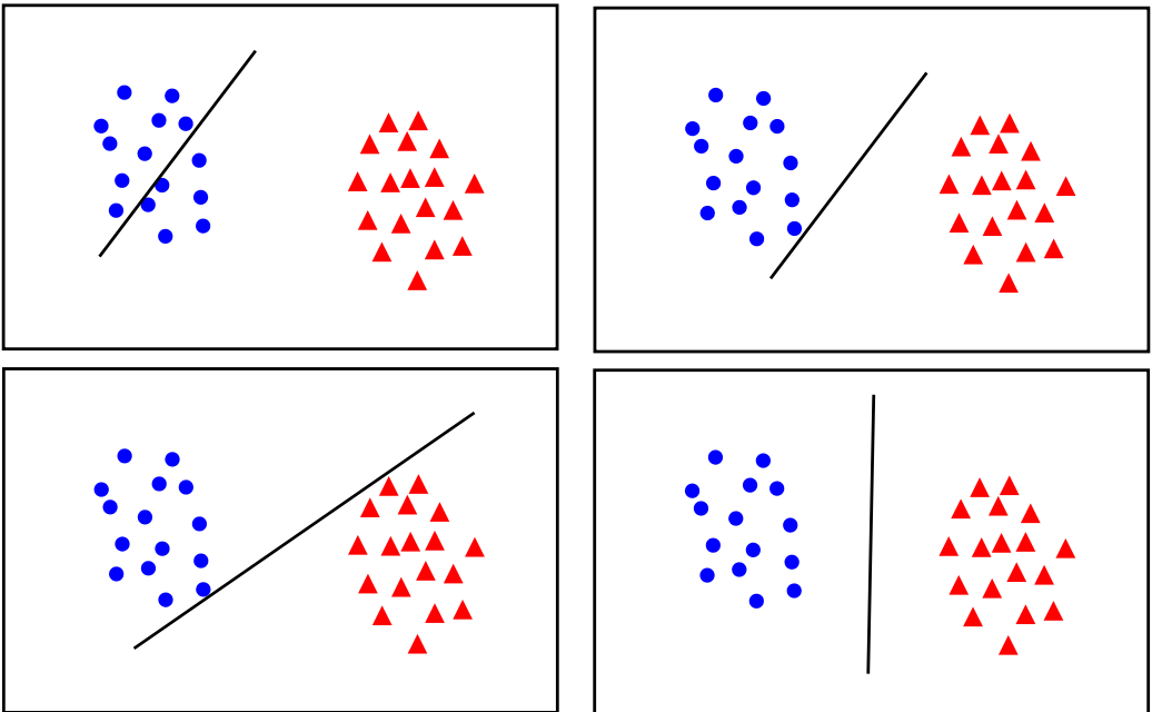
But hopefully by looking at these images, you can see what we should try to do. Instead of trying to fit all points lets focus on a few boundary points. Our aim will be to find a boundary between the classes that leads to the largest margin (buffer) from points on both sides.
What is an SVM?
An SVM is a set of three parallel hyperplanes which divide the group of points $\bold{x_i}$ for which $y_i = 1$ and $y_i = -1$ so that the distance between the hyperplane and the nearest point $\bold{x_i}$ from each class is maximised. This can be summarised really quite elegantly as the following function
$ f(\boldsymbol{x_i}) = \begin{cases} 1 & \text{if } \bold{x_i} \cdot \bold{w} + b \geq 1, \ -1 & \text{if } \bold{x_i} \cdot \bold{w} + b \leq -1, \ \text{Unknown Class} & \text{if } -1 < \bold{x_i} \cdot \bold{w} + b < 1. \end{cases} $
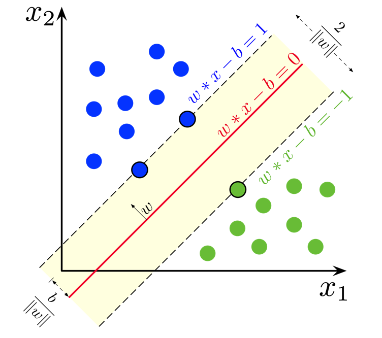
So, just like for logistic regression and linear regression, what we want to learn is just one set of weights $\bold{w}$ and a bias $b$. But this time we want the output $y = \bold{x_i w} + b$ to have some sense of a "margin" built in. A larger margin indicates that our predictions are more confident. The points that lie on the decision boundaries are what we call our support vectors because they're used to calculate the margin.
For prediction, the unknown class can be represented as a new number (e.g, $0$), but often after training people will just get rid of the unknown class and decide the class purely based on the sign of the linear function - or in terms of the diagram, on which side of the red line the point falls. This is entirely a matter of personal preference.
You'll notice here, in earlier chapters, in later chapters, and in the general literature that the way we multiply matrices is not very consistent. You might sometimes see $y = \bold{w x} + b$, $y = \bold{w^T x} + b$, $y = \bold{x w} + b$. Worse, sometimes the multiplication operation isn't clear, and $\cdot$ or $*$, might be used to represent matrix multiplication, the dot product, or even element-wise multiplication. The truth is, in large part it doesn't really matter. These all just stem from decisions of how we want to represent our data as matrices and vectors, and if we stay consistent in a project then everything is equivalent. Ideally academic papers will explicitly tell you the dimensions they're working with, like $\bold{x_i} \in \mathbb{R}^{5 \times 6}$, but especially for really large models it's anyone's guess 😂. The place where it really does matter is for performance, since the shape of matrices can have major implications on how quickly you can compute their product due to cache locality and all sorts of other reasons.
Loss Function
To train our weights and bias, we'll use gradient descent like we have done many times before. However, we'll introduce a new loss function, Hinge Loss,
$ \mathcal{L} = \begin{cases} 0 & \text{if } y_i \cdot f(x_i) \geq 1, \ 1 - y_i \cdot f(x_i) & \text{otherwise}. \end{cases} = \max{(0, 1 - y_i f(x_i))} $
Here, we can see that the loss is 0 if the predicted value $f(x_i)$ and the actual value $y_i$ are of the same sign ($y_i f(x_i) > 0$) and if the prediction falls outside the margin ($y_i f(x_i) >= 1$). Otherwise, we calculate the loss value $1 - y_i f(x_i)$ which will always be positive in the case of an incorrect prediction.
Regularisation
Unfortunately, once we start dealing with real data, we'll often find that our classes are not so distinct as we've seen in previous diagrams. Rather, you might have some noise and some mixing between the classes. As it stands, our SVM will priortise drawing a boundary that completely separates the two classes, rather than one which creates a large boundary. But in general, there's a trade off between the margin and the number of "mistakes" in the training data.
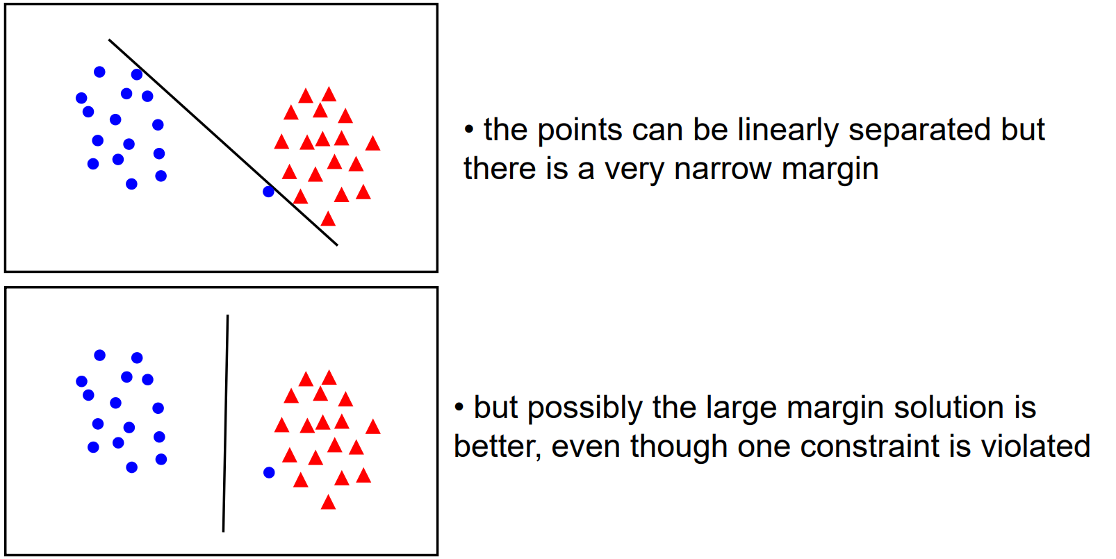
So, to allow us to control how "soft" or "hard" our boundary should be, we add a regularisation parameter to our loss function.
$ \mathcal{L} = \lambda ||\bold{w}||^2 + \max{(0, 1 - y_i f(x_i))} $
Geometrically, the distance between the margin hyperplanes is $\frac{2}{||\bold{w}||}$, so maximising the distance is equivalent to minimising $||\bold{w}||$.
Thus, high values of $\lambda$ will priortise a larger margin between the classes and a softer penalty for incorrect classification, whereas smaller values of $\lambda$ will prioritise giving the correct classification on the training data.
Gradient Descent
Generally, SVM is performed with Stochastic Gradient Descent - that is, our weights and bias are updated when calculating the loss for each sample. Since our loss has two clear cases, it's easiest to derive our gradients for gradient descent by considering them seperately.
Case 1: if $y_i f(x_i) >= 1$ (prediction is correct)
$ \mathcal{L}' (w, b) = \begin{bmatrix} \frac{\partial \mathcal{L}}{\partial w} \newline \frac{\partial \mathcal{L}}{\partial b} \end{bmatrix} = \begin{bmatrix} 2 \lambda w \newline 0 \end{bmatrix} $
Case 2: Otherwise (prediction is incorrect)
$ \mathcal{L}' (w, b) = \begin{bmatrix} \frac{\partial \mathcal{L}}{\partial w} \newline \frac{\partial \mathcal{L}}{\partial b} \end{bmatrix} = \begin{bmatrix} 2 \lambda w - y_i x_i \newline y_i \end{bmatrix} $
Exercise
Your task is to implement a linear binary Support Vector Machine classifier. You must implement fit() which adjusts the weights and bias of your model to some training data, predict() which returns the predicted classes of of an array of data points.
Inputs - fit():
Xis a NumPy NDArray (matrix) of data points such as[[1, 1, 0], [0, 0.5, 3], [0.7, 0.9, 0.3]], representing the training data.yis a NumPy NDArray (vector) of values such as[0, 1, 1], representing the corresponding (binary) class for each data point.
Inputs - predict():
Xis a NumPy NDArray (matrix) of data points such as[[1, 1, 0], [0, 0.5, 3], [0.7, 0.9, 0.3]], representing a set of points we want to predict a class for.
Extra Reading: SVM Formulations
Much like Linear Regression, there are many, many techniques for computing the SVM and we only showed one here today. Broadly, most of these can be categorised as solving the primal problem or the dual problem, which relates to how we frame the optimisation of the loss function. There are also some more modern approaches, but we can't really cover them here since the background knowledge needed is extensive. If you feel inclined though, Wikipedia is your friend!
The interesting point is that the difference in performance between these methods is not that great. Chapelle et al. showed in fact that both methods for solving the primal problem and the dual problem are $O(n^3)$ in complexity, with $n$ being the number of data points. However, the development of these different methods has allowed us to understand the problem of classification in much greater detail and discover more about SVMs.
Extra Reading: Non-linear Data & The Kernel Trick
Currently, the line (or hyperplane) of our SVM is pretty straight (or flat), so how would we find a decision boundary for a dataset like this?
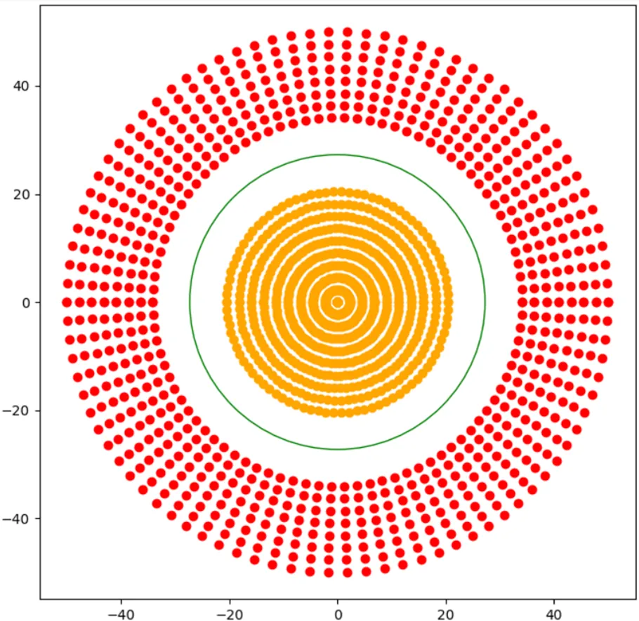
Recall that from the perceptron, we handled this sort of problem by introducing a non-linear activation function, but we can't do that here because our plane is inherently a linear expression.
Instead, what we can do is extend our data into a new non-linear dimension, and then find a hyperplane within that which separates our classes.
For instance, for every data point $(x_1, x_2)$ I could pipe it through the transformation $\phi: \mathbb{R}^{2 \times 1} \rightarrow \mathbb{R}^{3 \times 1}, \quad (x_1, x_2) \mapsto \left(x_1, x_2, \sqrt{x_1^2 + x_2^2}\right)$
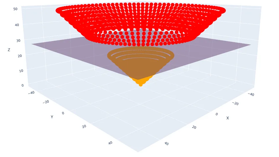
And now clearly I can draw a hyperplane between the two classes using my ordinary SVM methods.
Unfortunately, it can be very difficult to pick the best transformation, and if we decide to use several then our problem because very computationally expensive. One thing that helps us with this is called the kernel trick. This basically relies on the fact that to solve the dual problem, we don't need to know the result of the transformation for each point, we just need to know its similarity to other points under the same transformation. Chapelle et al. also demonstrated that this technique can be applied to solving the primal problem, but it's incredibly involved.
Extra Reading: Multiclass SVMs
In this chapter, we've only focussed on binary classification, and so you might be wondering if just like how logistic regression has a multiclass cousin in softmax regression, is there a multiclass version of SVMs? Fortuantely, there are two very intuitive approaches to solving this problem.
Firstly, there's the one-vs-one approach. For all pairs of k classes in our dataset, $\binom{k}{2}$, we create an SVM. Then we run our data point through all of these classifiers and pick the class with majority votes.
For example, considering 3 classes, we'd need 3 classifiers - 1 vs 2, 2 vs 3, and 1 vs 3. If the output for a datapoint fed into 1 vs 2 is class 1; 2 vs 3 is class 2; 1 vs 3 is class 1, the majority vote is class 1, which is our final result.
Secondly, there's the one-vs-all approach. For all k classes in our dataset, we create an SVM for that class vs any other data point not in it. Then, just like before, we run our data point through all the classifiers and pick the class with majority votes.
For example, considering 3 classes, we'd need 3 classifiers - 1 vs 2/3, 2 vs 1/3, and 3 vs 1/2. If the outputfor a datapoint fed into 1 vs 2/3 is class 1; 2 vs 1/3 is class 1 or class 3; 3 vs 1/2 is class 1 or class 2, then majority votes go to class 1, so that's our final result.
Welcome!
⚠️ In Progress! ⚠️
Welcome!
⚠️ In Progress! ⚠️
Welcome!
⚠️ In Progress! ⚠️
Welcome!
⚠️ In Progress! ⚠️
Welcome!
⚠️ In Progress! ⚠️
Welcome!
⚠️ In Progress! ⚠️
Deep Learning
Welcome!
⚠️ In Progress! ⚠️
Welcome!
⚠️ In Progress! ⚠️
Welcome!
⚠️ In Progress! ⚠️
Welcome!
⚠️ In Progress! ⚠️
Welcome!
⚠️ In Progress! ⚠️
Welcome!
⚠️ In Progress! ⚠️
Welcome!
⚠️ In Progress! ⚠️
Welcome!
⚠️ In Progress! ⚠️
Welcome!
⚠️ In Progress! ⚠️
Welcome!
⚠️ In Progress! ⚠️
Welcome!
⚠️ In Progress! ⚠️
Welcome!
⚠️ In Progress! ⚠️
Welcome!
⚠️ In Progress! ⚠️
Welcome!
⚠️ In Progress! ⚠️
Deep Learning
Welcome!
⚠️ In Progress! ⚠️
Welcome!
⚠️ In Progress! ⚠️
Welcome!
⚠️ In Progress! ⚠️
Welcome!
⚠️ In Progress! ⚠️
Welcome!
⚠️ In Progress! ⚠️