Naive Bayes Classifier
What's the Problem?
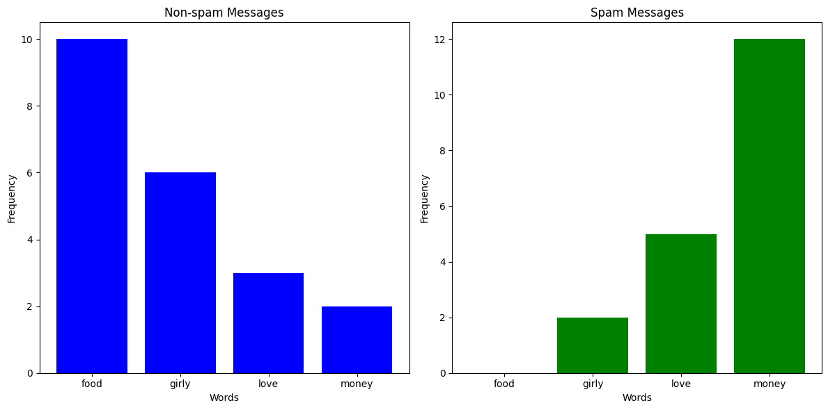
You've been getting a lot more spam bots texting you lately, and instead of blocking them manually, you've decided to build a classifier which can automatically predict whether a message is spam or not. You've noticed that messages from spam bots tend to have different vocabulary compared to what your friends send you, so you take a sample of messages and plot how many times certain words appear.

Clearly, if some words appear more than others, it is more likely that the message is from a spam bot. So, could we build a probabilistic classifier around that?
What is a Naive Bayes Classifier?
The idea behind Naives Bayes Classifiers is actually quite simple. Let's say we had \(K\) classes and \(n\) features, then if we assigned probabilities \(p(C_k | x_1, ..., x_n)\) to each class \(C_k\) given we have some feature vector \(\textbf{x} = (x_1, ..., x_n)\), then the model's best prediction would just be the class with the highest probablitiy.
For example, let's say we got a text with 4 occurences of the word "food", 2 occurences of the word "girly", 6 occurences of the word "love", and 0 occurrences of the word "money". We could represent that text as a vector \(\textbf{x} = (4, 2, 6, 0)\). Now, let's say that \(p(\text{Spam Message} | \textbf{x}) = 0.19\) and \(p(\text{Non-spam Message} | \textbf{x}) = 0.6\), then we would confidently say that the message is not spam.
The problem is how do we work out \(p(C_k | \textbf{x})\)? Fortunately, Bayes' Theorem comes to the rescue, because it tells us the conditional probabilitiy can be expressed as
\[ p(C_k | \textbf{x}) = \frac{p(C_k) p(\textbf{x} | C_k)}{p(\textbf{x})} \]
Often in Bayesian probability, the above equation will also be phrased as follows
\[ \text{posterior} = \frac{\text{prior} \times \text{likelihood}}{\text{evidence}} \]
We notice that for all \(C_k\), the denominator \(p(\textbf{x})\) doesn't change, so it's effectively a constant. Since we don't really care about the actual probability values but rather the predictions, we can just get rid of it for now to simplify our equations.
\[ p(C_k | \textbf{x}) \propto p(C_k) p(\textbf{x} | C_k) \]
\(\propto\) is the "proportional to" symbol, since strictly speaking the terms aren't equal
Now, by using the chain rule repeatedly and by assuming that each of the features of \(\textbf{x}\) are independent (see here for details), we can get the following expression
\[ p(C_k | \textbf{x}) \propto p(C_k)\prod_{i=1}^{n}p(x_i|C_k) \]
That means, with some feature vector \(\textbf{x}\), our prediction \(\hat{y}\) will be
\[ \hat{y} = \underset{k \in \{0, ..., K\}}{\text{argmax}} p(C_k)\prod_{i=1}^{n}p(x_i|C_k) \]
Sometimes, however, some probabilities will be so small that the actual numbers risk underflowing on a computer, causing weird undefined behaviour. For that reason, some models will just take the log probability of everything.
\[ \hat{y} = \underset{k \in \{ 0, ..., K \}}{\text{argmax}} \log{(p(C_k))} + \sum_{i=1}^{n} \log{(p(x_i|C_k))} \]
Types of Naive Bayes Classifier
There are many different types of Naive Bayes Classifiers depending on what sort of probability distributions the feature variables are sampled from.
- Bernoulli Naive Bayes: This is used with vectors with Boolean variables, such as \(\textbf{x} = (1, 1, 0, 0, 1)\).
- Multinomial Naive Bayes: This is used with features from multinomial distributions. This is especially useful for non-negative discrete data, such as frequency counts. The above examples of counting words in a text message are a good example of this. Here, if the probability of seeing the word in a text message given a certain class is \(p_k\), the likelihood of it appearing \(c\) times would be \(p_k^c\).
- Gaussian Naive Bayes: This is used with Gaussian/normal distributions. Typically when our feature variables are continuous, we assume that they're sampled from a gaussian distribution, and we thus calculate the likelihood \(p(x_i | C_k)\) as follows
\[ p(x_i | C_k) = \frac{1}{\sqrt{2 \pi \sigma_k^2}}e^{-\frac{(x_i - \mu_k)^2}{2 \sigma_k^2}} \]
- \(\sigma_k^2\) is the variance of \(x_i\) associated with the class \(C_k\)
- \(\mu_k\) is the mean of \(x_i\) associated with the class \(C_k\)
Alpha Value
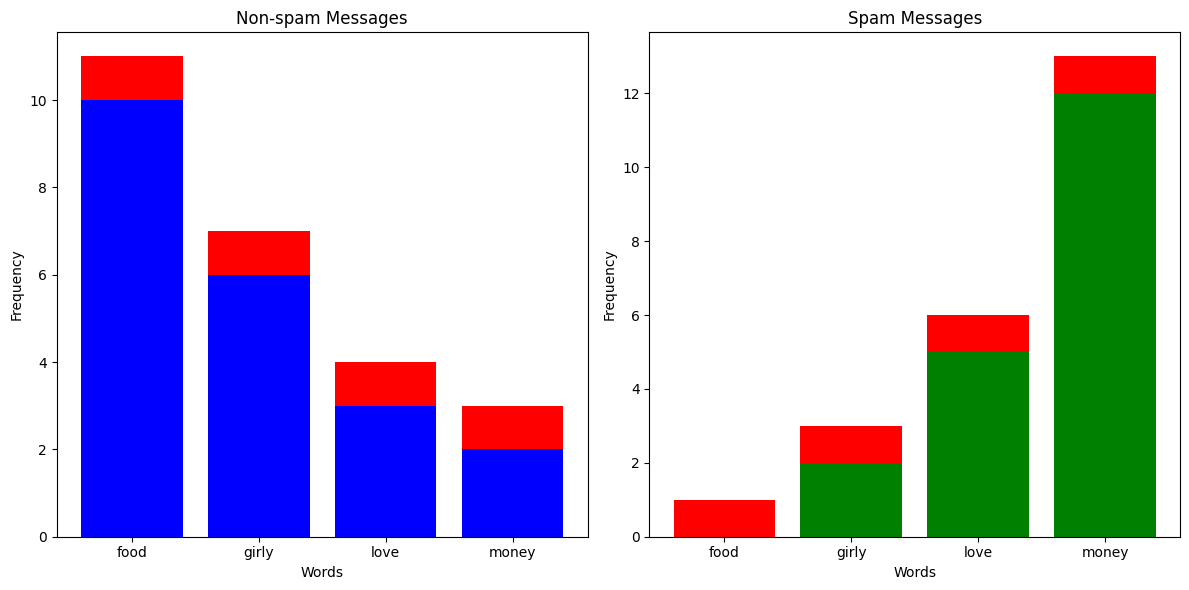
Let's say you've received a text message with 20 occurrences of the word "money" and 1 occurrence of the word "food". Just looking at the column chart above, you'd expect that the text message would be labelled as spam. But since there aren't any spam messages in the training data with the word "food", the likelihood of having 1 occurrence in a spam message is 0, meaning \(p(\text{Spam Message} | (1, 0, 0, 20)) = 0\). This is clearly a problem, so what we do is something called Laplace smoothing. Effectively, we add an \(\alpha\) to all the occurences of everything in our training set to avoid multiplying anything by 0.

Exercise
Multinomial Classifier
Your task is to implement a Multinomial Naive Bayes Classifier. You must implement fit() which takes training data and preprocesses it for predictions, and _predict() which returns the predicted class for a given feature vector. You should account for an \(\alpha\) value, but you should not use \(\log\) probabilities.
Inputs - fit():
Xis a NumPy NDArray (matrix) of feature vectors sampled from a multinomial distribution that form your training data. For example,[[1, 1, 0, 1], [2, 3, 4, 1], [3, 4, 2, 1]]. In context of the spam filter, you could imagine each inner as a counter for a text message, with each number representing the occurences of a certain word.yis a NumPy NDArray (vector) representing the classes of each feature vector ofX. For example,[0, 0, 1]. In context of the spam filter, you could imagine each number corresponding to a True/False of whether each corresponding text message is spam.alphais a non-negative integer representing the Laplace smoothing parameter. This represents how much you should add to each feature count per class for calculating likelihood.
Inputs - _predict():
xis a NumPy NDArray (vector) representing a feature vector sampled from a multinomial distribution which you should predict the class of from the training data. For example,[1, 2, 0, 1].
Gaussian Classifier
Your task is to implement a Gaussian Naive Bayes Classifier. You must implement fit() which takes training data and preprocesses it for predictions, and _predict() which returns the predicted class for a given feature vector. You do not need to account for an \(\alpha\) value, but you should use \(\log\) probabilities.
Inputs - fit():
Xis a NumPy NDArray (matrix) of feature vectors with continuous values that form your training data. For example,[[23.4, 11.2, 1.2], [4.3, 5.6, 1.2], [3.3, 2.2, 14.2]]. For some context, you could imagine each inner array as some summary of a customer, and each value as the average number of minutes spent in certain stores.yis a NumPy NDArray (vector) representing the classes of each feature vector ofX. For example,[2, 0, 1]. In the same context, these labels could refer to whether the customer is "non-binary, male, female".
Inputs - _predict():
xis a NumPy NDArray (vector) representing a feature vector with continuous values which you should predict the class of from the training data. For example,[1.2, 1.1, 6.3].
Extra Reading: What is so naive?
Remember that at the basic level, a Naive Bayes Classifier wants to find the \(p(C_k | \textbf{X})\) with the greatest value. To calculate this, it needs to calculate \(p(\textbf{x} | C_k)\). However, because this value is generally hard to calculate, we make a big assumption that the features of \(\textbf{x}\) are independent, so we can end up with the formula \(p(\textbf{x} | C_k) = p(x_1 | C_k) \times p(x_2 | C_k) \times p(x_3 | C_k) \times \dots\). It's this assumption that we call naive, because it may or may not turn out to be correct.
There is actually a fantastic intuitive explanation of this on Wikipedia
All naive Bayes classifiers assume that the value of a particular feature is independent of the value of any other feature, given the class variable. For example, a fruit may be considered to be an apple if it is red, round, and about 10 cm in diameter. A naive Bayes classifier considers each of these features to contribute independently to the probability that this fruit is an apple, regardless of any possible correlations between the color, roundness, and diameter features.
Of course, very often this assumption is incorrect, but even in those cases, Naive Bayes Classifiers can still perform remarkably well. In fact, they can even outperform models that don't make such an assumption because they can avoid some of the pitfalls of the curse of dimensionality. For example, if two features are dependent, such as hair length and gender, then assuming independence lets you double count the evidence, which is especially helpful when you're dealing with many, many features.
A more mathematical explanation for Naive Bayes effectiveness can be found in research, but the explanations get quite a bit more involved.